How to deal with right-censored observations
I’ve recently been interested in understanding survival models, which model the time to an event of interest (tte) but where we are not always able to wait until that event occurs. This happens, for example, when modelling the time until a customer churns: some of your customers may have cancelled their subscriptions but many hopefully haven’t. Those that haven’t are said to be censored because we haven’t observed them cancel their subscription yet.
As a first step in that direction, we’ll take a look at modelling censoring when the tte has a Poisson distribution (minor modifications can be made to extend to other distributions). We’ll use Stan to implement our model since Bayesian notation very nicely reflects our statistical understanding. Don’t worry if you aren’t familiar with Stan or Bayesian inference - it should be possible to follow along regardless.
You can download the R markdown and the stan model to try it out.
Some theory
The Problem
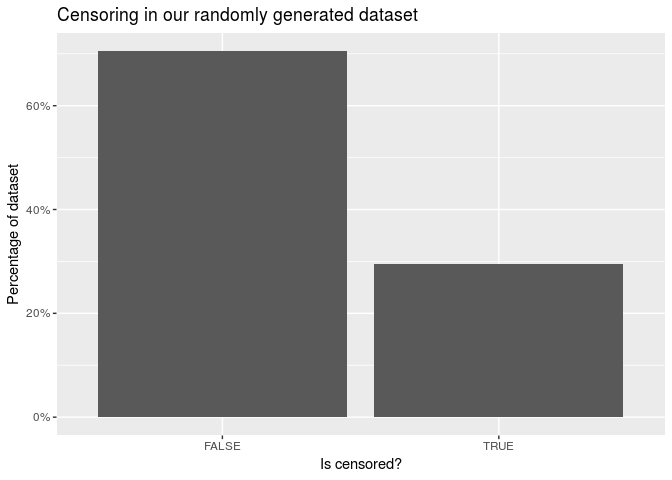
Let’s generate some data. We will assume that the time to event (tte) is poisson distributed with mean \(\mu = 10\). However, we will also assume that we don’t get to observe the event of interest in every case, i.e. some cases are censored. What we measure is the time to observation (tto).
N <- 10000
mu <- 10

df <- tibble(
  id = 1:N,
  tte = rpois(N, mu),
  tto = pmin(rpois(N, 12), tte),
  censored = tto < tte
)

df %>%
  head() %>%
kable() %>% kable_styling()| id | tte | tto | censored |
|---|---|---|---|
| 1 | 12 | 11 | TRUE |
| 2 | 7 | 7 | FALSE |
| 3 | 4 | 4 | FALSE |
| 4 | 13 | 8 | TRUE |
| 5 | 10 | 10 | FALSE |
| 6 | 15 | 8 | TRUE |
Note that we observe tto but not tte. How might we estimate \(\mu\)? One way is to take the mean.
df %>%
  select(tte, tto) %>%
  summarise_all(mean) %>%
kable() %>% kable_styling()| tte | tto |
|---|---|
| 9.9916 | 8.9525 |
This estimate is fairly good for tte but is too low for tto. This was to be expected because we know that tto is smaller than tte for censored observations.
It’s not possible to just filter out the censored values as this also gives biased estimates. In fact, it makes our estimate worse in this case.
df %>%
  filter(!censored) %>%
  select(tte, tto) %>%
  summarise_all(mean) %>%
kable() %>% kable_styling()| tte | tto |
|---|---|
| 8.916655 | 8.916655 |
A more sophisticated way to be wrong
So how can we estimate μ using just tto? The first step is to reinterperet the mean as the estimator that maximises a likelihood (the maximum likelihood estimator, or MLE). The likelihood is defined as the probability of the data given the estimate. Under the true model, this probability is \(f(tte_i \mid \mu) = \text{Poisson}(tte_i \mid \mu)\) for the \(i\)th case, giving the likelihood of the whole dataset as:
\[ L(\mu) := \prod_{i = 1}^N f(tte_i | \mu) . \]
The mean maximises this likelihood, which is why the mean of tte is close to the true value.
To further illustrate this point, note that this is the estimate we get when regressing tte on a constant.
df %>%
  glm(
    formula = tte ~ 1,
    family = poisson(link = 'log'),
    data = .
  ) %>%
  tidy() %>%
  pull(estimate) %>%
  exp()
[1] 9.9916However, we don’t observe tte; we observe tto. Simply replacing tte with tto and maximising
\[ L(\mu) := \prod_{i = 1}^N f(tto_i \mid \mu) \]
gives us the mean of tto, which is a bad estimate because this ‘likelihood’ does not take censoring into account.
The correct likelihood
So what likelihood can we use? Note that in uncensored cases, \(f(tto_i \mid \mu) = f(tte_i \mid \mu)\), just like above.
In the censored cases, all we know is that tte must be larger than what was observed. This means that we need to sum over the probabilities of all possibilities: \(S(tto_i \mid \mu) := \sum_{t > tto_i} f(t \mid \mu)\). The full likelihood is then
\[ L(\mu) := \prod_{i = 1}^N \delta_i f(tto_i \mid \mu) \times \prod_{i = 1}^N (1 - \delta_i) S(tto_i \mid \mu) , \]
where \(\delta_i\) is 1 if the event was observed and 0 if censored. Although we’ll stick to the Poisson model in this post, we can use these ideas to create a likelihood for many different choices of distribution by using the appropriate probability/survival functions \(f\), \(S\).
Implementation
We will fit this model using Stan because it is relatively easy to write a Bayesian model once we have understood the data generating process. This will require us to define prior distributions (on \(\mu\)) just like with any Bayesian method. Since we are mostly interested in understanding the likelihood here, we will not give much consideration to the prior. However, if applying this to a real problem, it would be a good idea to give this more thought in a principled Bayesian workflow.
Terminology
Stan makes the following abbreviations:
pmf- probability mass function, \(f(tto_i \mid \mu) = \text{Poisson}(tto_i \mid \mu)\)
lpmf- log(
pmf) ccdf- survival function, a.k.a. complementary cumulative distribution function, \(S(tto_i | \mu) := \sum_{t > tto_i} \text{Poisson}(t | \mu)\)
lccdf- log(
ccdf) target- log(posterior probability density) = log(likelihood x prior).
Stan uses the log-scale for its calculations, so we will need the log-likelihood:
\[ \log L(\mu) := \sum_{i = 1}^N \delta_i \log f(tto_i \mid \mu) + \sum_{i = 1}^N (1 - \delta_i) \log S(tto_i \mid \mu) . \]
The model
In our model, we add the lccdf if the observation is censored and lpmf if not censored. Let’s load our model and take a look.
model <- stan_model('censored_poisson.stan')modelS4 class stanmodel 'censored_poisson' coded as follows:
data {
// the input data
int<lower = 1> n; // number of observations
int<lower = 0> tto[n]; // tto is a list of ints
int<lower = 0, upper = 1> censored[n]; // list of 0s and 1s
// parameters for the prior
real<lower = 0> shape;
real<lower = 0> rate;
}
parameters {
// the parameters used in our model
real<lower = 0> mu;
}
model {
// posterior = prior * likelihood
// prior
mu ~ gamma(shape, rate);
// likelihood
for (i in 1:n) {
if (censored[i]) {
target += poisson_lccdf(tto[i] | mu);
} else {
target += poisson_lpmf(tto[i] | mu);
}
}
} The language used in the Stan model is slightly different from R-notation but hopefully intuitive enough to convince yourself that it’s the same model we described above.
Now we can sample from the posterior of our model.
fit <- model %>%
  sampling(
    data = compose_data(df, shape = 2, rate = 0.05),
    iter = 2000,
    warmup = 500
  )

fit
Inference for Stan model: censored_poisson.
4 chains, each with iter=2000; warmup=500; thin=1;
post-warmup draws per chain=1500, total post-warmup draws=6000.
mean se_mean sd 2.5% 25% 50% 75%
mu 9.98 0.00 0.03 9.92 9.96 9.98 10.01
lp__ -19613.55 0.01 0.69 -19615.54 -19613.71 -19613.29 -19613.09
97.5% n_eff Rhat
mu 10.05 2002 1
lp__ -19613.04 2924 1
Samples were drawn using NUTS(diag_e) at Sat Aug 4 15:49:36 2018.
For each parameter, n_eff is a crude measure of effective sample size,
and Rhat is the potential scale reduction factor on split chains (at
convergence, Rhat=1).Stan has an amazing array of diagnostics to check the quality of the fitted model. Since our model is fairly simple and all checks are in order, I won’t describe them here.
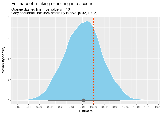
The point estimate for mu is 9.98 and the true value is contained within the 95% credible interval [9.92, 10.05]. We can also plot all the samples from our posterior.
Conclusion
We have seen how to change the likelihood to take censored observations into account. Moreover, the same process works for most distributions, so you can swap out the Poisson for Weibull/gamma/lognormal or whatever you want. Using the Bayesian modelling language, Stan, makes it super easy to test your statistical intuitions by turning them into a workable model, so I’ll definitely be exploring Stan more in the future.