Hierarchical Customer Lifetime Value
In a previous post, we described how a model of customer lifetime value (CLV) works, implemented it in Stan, and fit the model to simulated data. In this post, we’ll extend the model to use hierarchical priors in two different ways: centred and non-centred parameterisations. I’m not aware of any other HMC-based implementations of this hierarchical CLV model, so we’ll run some basic tests to check it’s doing the right thing. More specifically, we’ll fit it to a dataset drawn from the prior predictive distribution. The resulting fits pass the main diagnostic tests and the 90% posterior intervals capture about 91% of the true parameter values.
A word of warning: I came across a number of examples where the model showed severe E-BFMI problems. This seems to happen when the parameters \(\mu\) (inverse expected lifetime) and \(\lambda\) (expected purchase rate) are fairly similar, but I haven’t pinned down a solid reason for these energy problems yet. I suspect this has something to do with the difficulty in distinguishing a short lifetime from a low purchase rate. This is a topic we’ll leave for a future post.
We’ll work with raw stan, which can be a bit fiddly sometimes. To keep this post within the limits of readability, I’ll define some custom functions to simplify the process. Check out the full code to see the details of these functions.
\(\DeclareMathOperator{\dbinomial}{Binomial}\DeclareMathOperator{\dbernoulli}{Bernoulli}\DeclareMathOperator{\dpoisson}{Poisson}\DeclareMathOperator{\dnormal}{Normal}\DeclareMathOperator{\dt}{t}\DeclareMathOperator{\dcauchy}{Cauchy}\DeclareMathOperator{\dexponential}{Exp}\DeclareMathOperator{\duniform}{Uniform}\DeclareMathOperator{\dgamma}{Gamma}\DeclareMathOperator{\dinvgamma}{InvGamma}\DeclareMathOperator{\invlogit}{InvLogit}\DeclareMathOperator{\logit}{Logit}\DeclareMathOperator{\ddirichlet}{Dirichlet}\DeclareMathOperator{\dbeta}{Beta}\)
Data Generating Process
Let’s recap on the story from last time. We have a 2-year old company that has grown linearly over that time to gain a total of 1000 customers.
set.seed(65130) # https://www.random.org/integers/?num=2&min=1&max=100000&col=5&base=10&format=html&rnd=new

customers <- tibble(id = 1:1000) %>%
  mutate(
    end = 2 * 365,
    start = runif(n(), 0, end - 1),
    T = end - start
  )
Within a customer’s lifetime \(\tau\), they will purchase with Poisson-rate \(\lambda\). We can simulate the time \(t\) till last observed purchase and number of purchases \(k\) with sample_conditional.
sample_conditional <- function(T, tau, lambda) {

  # start with 0 purchases
  t <- 0
  k <- 0

  # simulate time till next purchase
  wait <- rexp(1, lambda)

  # keep purchasing till end of life/observation time
  while(t + wait <= pmin(T, tau)) {
    t <- t + wait
    k <- k + 1
    wait <- rexp(1, lambda)
  }

  # return tabular data
  tibble(
    t = t,
    k = k
  )
}

s <- sample_conditional(300, 200, 1) | t | k |
|---|---|
| 198.2929 | 169 |
In the above example, even though the observation time is \(T = 300\), the time \(t\) till last purchase will always be below the lifetime \(\tau = 200\). With a purchase rate of 1 per unit time, we expect around \(k = 200\) purchases.
Model
We’ll use the same likelihood as before, which says that the probability of customer \(i\)’s data given their parameters is
\[ \begin{align} \mathbb P(k, t, T \mid \mu_i, \lambda_i) &= \frac{\lambda_i^k}{\lambda_i + \mu_i} \left( \mu_i e^{-t(\lambda_i + \mu_i)} + \lambda_i e^{-T(\lambda_i + \mu_i)} \right) \\ &\propto p \dpoisson(k \mid t\lambda_i)S(t \mid \mu_i) \\ &\hphantom{\propto} + (1 - p) \dpoisson(k \mid t\lambda_i)\dpoisson(0 \mid (T-t)\lambda_i)S(T \mid \mu_i) , \\ p &:= \frac{\mu_i}{\lambda_i + \mu_i} , \end{align} \]
where \(S\) is the exponential survival function.
To turn this into a Bayesian model, we’ll need priors for the parameters. The last time, we put simple gamma priors on the parameters \(\mu_i\) and \(\lambda_i\). For example, we could choose \(\lambda_i \sim \dgamma(2, 28)\) if we were to use the simple model from last time (similarly for \(\mu_i\)). This time we’re going hierarchical. There are various ways to make this hierarchical. Let’s look at two of them.
One method arises directly from the difficulty of specifying the gamma-prior parameters. It involves just turning those parameters into random variables to be simultaneously estimated along with \(\mu_i\) and \(\lambda_i\). For example, we say \(\lambda_i \sim \dgamma(\alpha, \beta)\), where \(\alpha_i \sim \dgamma(\alpha_\alpha, \beta_\alpha)\) and \(\beta_i \sim \dgamma(\alpha_\beta, \beta_\beta)\) (and similarly for \(\mu_i\)). We eventually want to incorporate covariates, which is difficult with this parameterisation, so let’s move onto a different idea.
Another solution is to use log-normal priors. This means setting
\[ \begin{align} \lambda_i &:= \exp(\alpha_i) \\ \alpha_i &\sim \dnormal(\beta, \sigma) \\ \beta &\sim \dnormal(m, s_m) \\ \sigma &\sim \dnormal_+(0, s) , \end{align} \]
where \(m\), \(s_m\), and \(s\) are constants specified by the user (and similarly for \(\mu_i\)). This implies
- there is an overall mean value \(e^\beta\),
- the customer-level effects \(\alpha_i\) are deviations from the overall mean, and
- the extent of these deviations is controlled by the magnitude of \(\sigma\).
With \(\sigma \approx 0\), there can be very little deviation from the mean, so most customers would be the same. On the other hand, large values of \(\sigma\) allow for customers to be (almost) completely unrelated to each other. This means that \(\sigma\) is helping us to regularise the model.
The above parameterisation is called “centred”, which basically means the prior for \(\alpha_i\) is expressed in terms of other parameters (\(\beta\), \(\sigma\)). This can be rewritten as a “non-centred” parameterisation as
\[ \begin{align} \lambda_i &:= \exp(\beta + \sigma \alpha_i) \\ \alpha_i &\sim \dnormal(0, 1) \\ \beta &\sim \dnormal(m, s_m) \\ \sigma &\sim \dnormal_+(0, s) . \end{align} \]
Notice the priors now contain no references to any other parameters. This is equivalent to the centred parameterisation because \(\beta + \sigma \alpha_i \sim \dnormal(\beta, \sigma)\). The non-centred parameterisation is interesting because it is known to increase the sampling efficiency of HMC-based samplers (such as Stan’s) in some cases.
Centred Stan implementation
Here is a centred stan implementation of our log-normal hierarchical model.
centred <- here::here('models/rf_centred.stan') %>%
  stan_model()
Note that we have introduced the prior_only flag. When we specify that we want prior_only, then stan will not consider the likelihood and will instead just draw from the priors. This allows us to make prior-predictive simulations. We’ll generate a dataset using the prior-predictive distribution, then fit our model to that dataset. The least we can expect from a model is that it fits well to data drawn from its prior distribution.
Simulate the dataset
To simulate datasets we’ll use hyperpriors that roughly correspond to the priors from the previous post. In particular, the expected lifetime is around 31 days, and the expected purchase rate around once per fortnight.
data_hyperpriors <- list(
  log_life_mean_mu = log(31),
  log_life_mean_sigma = 0.7,
  log_life_scale_sigma = 0.8,

  log_lambda_mean_mu = log(1 / 14),
  log_lambda_mean_sigma = 0.3,
  log_lambda_scale_sigma = 0.5
)

data_prior <- customers %>%
  mutate(t = 0, k = 0) %>%
  tidybayes::compose_data(data_hyperpriors, prior_only = 1)

data_prior %>% str()
List of 14
$ id : int [1:1000(1d)] 1 2 3 4 5 6 7 8 9 10 ...
$ end : num [1:1000(1d)] 730 730 730 730 730 730 730 730 730 730 ...
$ start : num [1:1000(1d)] 328 707 408 342 666 ...
$ T : num [1:1000(1d)] 401.6 22.6 322.2 388.5 64.5 ...
$ t : num [1:1000(1d)] 0 0 0 0 0 0 0 0 0 0 ...
$ k : num [1:1000(1d)] 0 0 0 0 0 0 0 0 0 0 ...
$ n : int 1000
$ log_life_mean_mu : num 3.43
$ log_life_mean_sigma : num 0.7
$ log_life_scale_sigma : num 0.8
$ log_lambda_mean_mu : num -2.64
$ log_lambda_mean_sigma : num 0.3
$ log_lambda_scale_sigma: num 0.5
$ prior_only : num 1Let’s simulate 8 possible datasets from our priors. Notice how the centres and spreads of the datasets can vary.
centred_prior <- centred %>%
  fit( # a wrapper around rstan::sampling to allow caching
    file = here::here('models/rf_centred_prior.rds'), # cache
    data = data_prior,
    pars = c('customer'), # ignore this parameter
    include = FALSE,
    chains = 8,
    cores = 4,
    warmup = 1000, # not sure why this needs to be so high
    iter = 1001, # one more than warmup because we just want one dataset per chain
    seed = 3901 # for reproducibility
  )

centred_prior_draws <- centred_prior %>%
  get_draws( # rstan::extract but also with energy
    pars = c(
    'lp__', 'energy__',
    'theta',
    'log_centres',
    'scales'
    )
  ) %>%
  name_parameters() # add customer id, and idx = 1 (mu) or 2 (lambda)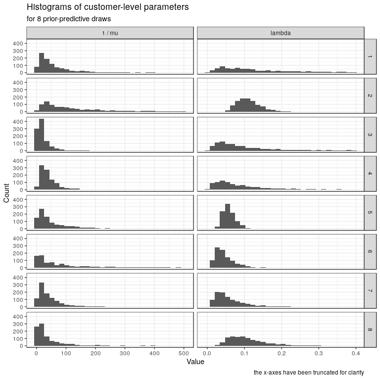
Here are the exact hyperparameters used.
hyper <- centred_prior_draws %>%
  filter(str_detect(parameter, "^log_|scales")) %>%
  select(chain, parameter, value) %>%
spread(parameter, value) | chain | log_centres[1] | log_centres[2] | scales[1] | scales[2] |
|---|---|---|---|---|
| 1 | 3.643546 | -2.057017 | 1.0866138 | 1.0874820 |
| 2 | 4.586349 | -2.231530 | 1.2064439 | 0.2725037 |
| 3 | 2.673924 | -2.475513 | 0.8847336 | 0.9429385 |
| 4 | 3.490525 | -2.557564 | 0.7708666 | 1.0124164 |
| 5 | 3.422691 | -2.877842 | 1.3232360 | 0.2920695 |
| 6 | 4.205884 | -3.196397 | 1.9217956 | 0.5307348 |
| 7 | 3.381881 | -2.995128 | 1.0299251 | 0.7266123 |
| 8 | 3.046531 | -2.328561 | 1.3993460 | 0.4751674 |
We’ll add the prior predictive parameter draws from chain 1 to our customers dataset.
set.seed(33194)

df <- centred_prior_draws %>%
  filter(chain == 1) %>%
  filter(name == 'theta') %>%
  transmute(
    id = id %>% as.integer(),
    parameter = if_else(idx == '1', 'mu', 'lambda'),
    value
  ) %>%
  spread(parameter, value) %>%
  mutate(tau = rexp(n(), mu)) %>%
  inner_join(customers, by = 'id') %>%
  group_by(id) %>%
  group_map(~sample_conditional(.$T, .$tau, .$lambda) %>% bind_cols(.x))

data_df <- data_hyperpriors %>%
tidybayes::compose_data(df, prior_only = 0)| id | t | k | lambda | mu | tau | end | start | T |
|---|---|---|---|---|---|---|---|---|
| 1 | 44.453109 | 44 | 0.8508277 | 0.0383954 | 44.669086 | 730 | 328.4312 | 401.56876 |
| 2 | 21.237790 | 5 | 0.2202757 | 0.0091300 | 263.541504 | 730 | 707.3906 | 22.60937 |
| 3 | 0.000000 | 0 | 0.0285432 | 0.0583523 | 8.405014 | 730 | 407.8144 | 322.18558 |
| 4 | 61.946272 | 7 | 0.0970620 | 0.0424386 | 71.617849 | 730 | 341.5465 | 388.45349 |
| 5 | 8.273831 | 3 | 0.1732173 | 0.0608967 | 8.747799 | 730 | 665.5210 | 64.47898 |
| 6 | 107.182661 | 19 | 0.1224131 | 0.0159025 | 113.792604 | 730 | 388.0271 | 341.97287 |
Fit the model to simulations
Now we can fit the model to the prior-predictive data df.
centred_fit <- centred %>%
  fit( # like rstan::sampling but with file-caching as in brms
    file = here::here('models/rf_centred_fit.rds'), # cache
    data = data_df,
    chains = 4,
    cores = 4,
    warmup = 2000,
    iter = 3000,
    control = list(max_treedepth = 12),
    seed = 24207,
    pars = c('customer'),
    include = FALSE
  )

centred_fit %>%
  check_hmc_diagnostics()
Divergences:
0 of 4000 iterations ended with a divergence.
Tree depth:
0 of 4000 iterations saturated the maximum tree depth of 12.
Energy:
E-BFMI indicated no pathological behavior.The HMC diagnostics pass. However, in some of the runs not shown here, there were pretty severe problems with the E-BFMI diagnostic (~0.01) and I’ve yet to figure out exactly which kinds of situations cause these energy problems. Let’s check out the pairwise posterior densities of energy with the hyperparameters.
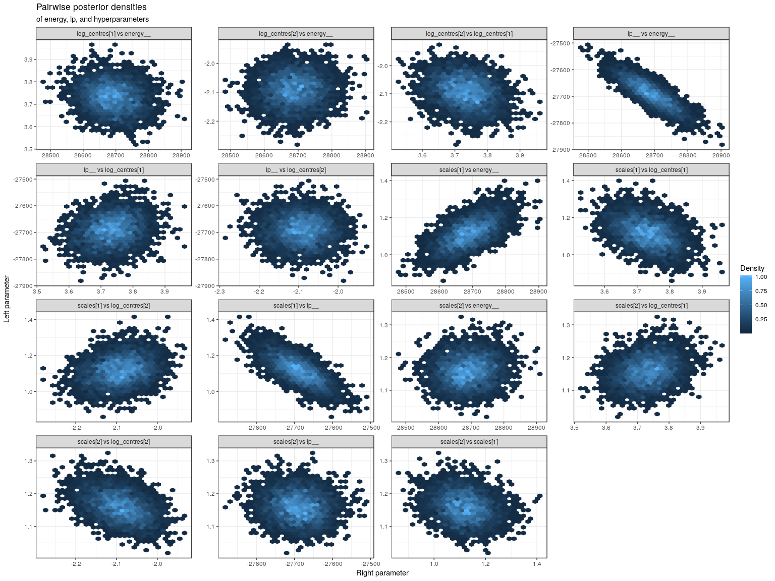
The scale parameter for the expected lifetime (scales[1]) is correlated with energy, which is associated with the energy problems described above. I’m not sure how much of a problem this poses, so let’s check out some more diagnostics.
neff <- centred_fit %>%
  neff_ratio() %>%
  tibble(
    ratio = .,
    parameter = names(.)
  ) %>%
  filter(ratio < 0.5) %>%
  arrange(ratio) %>%
head(20) | ratio | parameter |
|---|---|
| 0.0937772 | scales[1] |
| 0.1195873 | lp__ |
| 0.2592819 | log_centres[1] |
| 0.2748369 | scales[2] |
| 0.3228056 | log_centres[2] |
| 0.4340080 | theta[574,2] |
| 0.4381685 | theta[169,1] |
| 0.4800795 | theta[38,1] |
Both the lp__ and scales[1] parameters have low effective sample sizes. The rhat values seem fine though.
centred_rhat <- centred_fit %>%
  rhat() %>%
  tibble(
    rhat = .,
    parameter = names(.)
  ) %>%
  summarise(
    min_rhat = min(rhat, na.rm = TRUE),
    max_rhat = max(rhat, na.rm = TRUE)
) | min_rhat | max_rhat |
|---|---|
| 0.9990247 | 1.005071 |
Let’s now compare the 90% posterior intervals with the true values. Ideally close to 90% of the 90% posterior intervals capture their true value.
centred_cis <- centred_draws %>%
  group_by(parameter) %>%
  summarise(
    lo = quantile(value, 0.05),
    point = quantile(value, 0.50),
    hi = quantile(value, 0.95)
  ) %>%
  filter(!str_detect(parameter, '__')) # exclude diagostic parameters
The table below shows we managed to recover three of the hyperparameters. The scales[2] parameter was estimated slightly too high.
calibration_hyper <- hyper %>%
  filter(chain == 1) %>%
  gather(parameter, value, -chain) %>%
  inner_join(centred_cis, by = 'parameter') %>%
mutate(hit = lo <= value & value <= hi)| parameter | value | lo | point | hi | hit |
|---|---|---|---|---|---|
| log_centres[1] | 3.643546 | 3.6280113 | 3.733964 | 3.831287 | TRUE |
| log_centres[2] | -2.057017 | -2.1786705 | -2.090098 | -2.008663 | TRUE |
| scales[1] | 1.086614 | 0.9988373 | 1.119258 | 1.242780 | TRUE |
| scales[2] | 1.087482 | 1.0938685 | 1.160415 | 1.232225 | FALSE |
We get fairly close to 90% of the customer-level parameters.
true_values <- df %>%
  select(id, mu, lambda) %>%
  gather(parameter, value, -id) %>%
  mutate(
    idx = if_else(parameter == 'mu', 1, 2),
    parameter = str_glue("theta[{id},{idx}]")
  )

centred_calibration <- centred_cis %>%
  inner_join(true_values, by = 'parameter') %>%
  ungroup() %>%
  summarise(mean(lo <= value & value <= hi)) %>%
  pull() %>%
  percent()

centred_calibration
[1] "91.1%"This is slightly higher than the ideal value of 90%.
Non-centred Stan implementation
Here is a non-centred stan implementation of our log-normal hierarchical model. The important difference is in the expression for \(\theta\) and in the prior for \(\text{customer}\).
noncentred <- here::here('models/rf_noncentred.stan') %>%
  stan_model()
Since the non-centred and centred models are equivalent, we can also consider df as a draw from the non-centred prior predictive distribution.
noncentred_fit <- noncentred %>%
  fit( # like rstan::sampling but with file-caching as in brms
    file = here::here('models/rf_noncentred_fit.rds'), # cache
    data = data_df,
    chains = 4,
    cores = 4,
    warmup = 2000,
    iter = 3000,
    control = list(max_treedepth = 12),
    seed = 1259,
    pars = c('customer'),
    include = FALSE
  )

noncentred_fit %>%
  check_hmc_diagnostics()
Divergences:
0 of 4000 iterations ended with a divergence.
Tree depth:
0 of 4000 iterations saturated the maximum tree depth of 12.
Energy:
E-BFMI indicated no pathological behavior.Again, the HMC diagnostics indicate no problems. Let’s check the pairwise densities anyway.
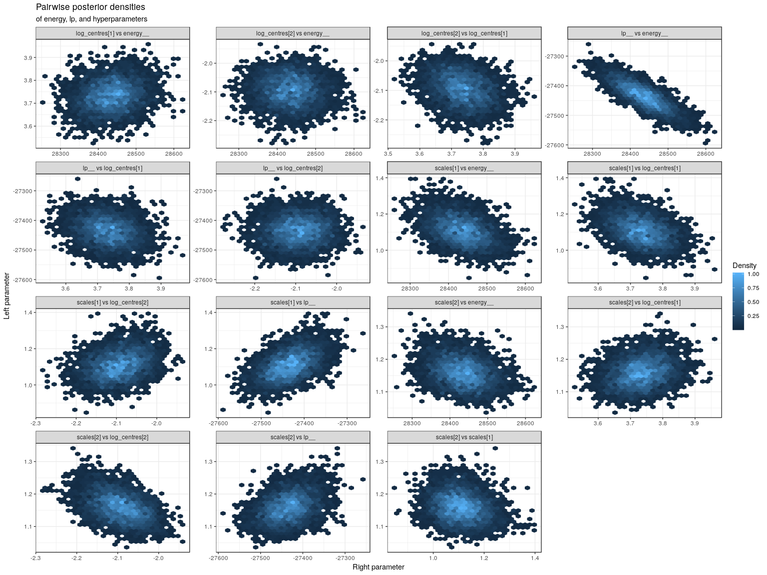
The correlation between scales[1] and energy__ is smaller with the non-centred parameterisation. This is reflected in the higher effective sample size for scales[1] below. Unfortunately, the effective sample size for the purchase rate hyperpriors has gone down.
neff <- noncentred_fit %>%
  neff_ratio() %>%
  tibble(
    ratio = .,
    parameter = names(.)
  ) %>%
  filter(ratio < 0.5) %>%
  arrange(ratio) %>%
head(20) | ratio | parameter |
|---|---|
| 0.0631821 | log_centres[2] |
| 0.0681729 | scales[2] |
| 0.1579867 | lp__ |
| 0.1776186 | scales[1] |
| 0.2217369 | log_centres[1] |
| 0.3910369 | theta[830,1] |
| 0.4767405 | theta[639,1] |
| 0.4792693 | theta[250,2] |
| 0.4847856 | theta[41,1] |
| 0.4978518 | theta[231,1] |
Again, the rhat values seem fine.
noncentred_rhat <- noncentred_fit %>%
  rhat() %>%
  tibble(
    rhat = .,
    parameter = names(.)
  ) %>%
  summarise(
    min_rhat = min(rhat, na.rm = TRUE),
    max_rhat = max(rhat, na.rm = TRUE)
) | min_rhat | max_rhat |
|---|---|
| 0.9990501 | 1.013372 |
Let’s check how many of the 90% posterior intervals contain the true value.
noncentred_cis <- noncentred_draws %>%
  group_by(parameter) %>%
  summarise(
    lo = quantile(value, 0.05),
    point = quantile(value, 0.50),
    hi = quantile(value, 0.95)
  ) %>%
  filter(!str_detect(parameter, '__'))
The hyperparameter estimates are much the same as with the centred parameterisation.
noncentred_calibration_hyper <- hyper %>%
  filter(chain == 1) %>%
  gather(parameter, value, -chain) %>%
  inner_join(noncentred_cis, by = 'parameter') %>%
mutate(hit = lo <= value & value <= hi)| parameter | value | lo | point | hi | hit |
|---|---|---|---|---|---|
| log_centres[1] | 3.643546 | 3.6325159 | 3.735363 | 3.838160 | TRUE |
| log_centres[2] | -2.057017 | -2.1770703 | -2.092537 | -2.014462 | TRUE |
| scales[1] | 1.086614 | 0.9970698 | 1.109297 | 1.235166 | TRUE |
| scales[2] | 1.087482 | 1.0963503 | 1.159626 | 1.234190 | FALSE |
About 91% of customer-level posterior intervals contain the true value.
noncentred_calibration <- noncentred_cis %>%
  inner_join(true_values, by = 'parameter') %>%
  summarise(mean(lo <= value & value <= hi)) %>%
  pull() %>%
  percent()

noncentred_calibration
[1] "91.0%"Discussion
Both centred and non-centred models performed reasonably well on the dataset considered. The non-centred model showed slightly less correlation between scales and energy__, suggesting it might be the better one to tackle the low E-BFMI problems. Since we only checked the fit on one prior-predictive draw, it would be a good idea to check out the fit to more draws. Some casual attempts of mine (not shown here) suggest there are situations that cause severe E-BFMI problems. Identifying these situations would be an interesting next step. It would also be great to see how it performs on some of the benchmarked datasets mentioned in the BTYDPlus package.