Selection bias in online experiments
After reading Judea Pearl’s Book of Why, I wanted to get to grips with causality in a familiar context: selection bias in online experiments and surveys. In such experiments, the cohorts are assigned randomly but we can only collect data on those users who actually log in and navigate to the section where the experiment has been set up. User engagement a possible and plausible confounder here, since your more engaged users are both more likely to log in and more/less enthusiastic about the particular change introduced in the experiment.
We’ll run a simulation in the context of measuring the click-through rate (CTR) of two cohorts, showing that selection bias can:
- give wrong estimates of the CTRs, and
- mask actual differences in the CTRs.
We’ll then rectify the above problems by defining a causal model and using the backdoor adjustment.
Feel free to download the Rmarkdown and try it out for yourself.
The problem
Let’s first show via simulation that it’s not possible to estimate the CTR of each cohort purely from the data. In the following section, we’ll show how to solve this problem by adding causal assumptions.
The data
We’ll assume that our list of users below is the population of interest and that we have segmented them by their levels of engagement. Both engagement and segment in the users dataset indicate the same information, where engagement is for convenience in our calculations and segment is for convenience of human-readability.
set.seed(6490418) # for reproducibility

n_users <- 500000

engagement_segments <- c('low', 'medium', 'high', 'very_high')

users <- tibble(id = 1:n_users) %>%
  mutate(
    cohort = rbinom(n_users, 1, 0.1),
    engagement = rbinom(n_users, 3, 0.15) - 1,
    segment = engagement_segments[engagement + 2] %>%
      ordered(levels = engagement_segments)
  )
In this situation, most of our users have a low level of engagement.

We then run our experiment and observe whether each user logged in (login), whether they viewed the particular section of the website where the experiment was taking place (viewed), and whether they clicked the button of interest (clicked). Included are also a couple of unobserved features: ctr, indicating the probability of that user clicking, and would_have_clicked, indicating whether the user would have clicked had they taken part in the experiment.
xp_complete <- users %>%
  mutate(
    login = rbinom(n_users, 1, inv_logit(engagement)) > 0,
    viewed = login & rbinom(n_users, 1, 0.5) > 0,
    ctr = inv_logit(-1 + engagement + engagement * cohort),
    would_have_clicked = rbinom(n_users, 1, ctr) > 0,
    clicked = viewed & would_have_clicked
  )
The engagement level is an integer between [-1, 2] (for convenience), which we map to a login probability via the inverse logit function. After logging in, the user will only take part in the experiment if they navigate to the correct page. If they do trigger a view in the experiment, the probability they also click is given as a (non-linear) function of engagement and cohort. The specific function used above assumes that more engaged users are more likely to click in general, and are also more likely to click if they are in cohort 1.
Without causal assumptions
We want to know which of the cohorts is more likely to click, regardless of whether they took part in this particular experiment. Thus, averaging would_have_clicked for each cohort will show us which is better overall. In this case, the large number of low-engagement users, who prefer cohort 0, tip the scales towards cohort 0.
actual <- xp_complete %>%
  group_by(cohort) %>%
  summarise(
    views = n(),
    clicks = sum(would_have_clicked),
    ctr = clicks / views
) | cohort | views | clicks | ctr |
|---|---|---|---|
| 0 | 449976 | 86476 | 0.1921791 |
| 1 | 50024 | 8155 | 0.1630217 |
The problem is that we don’t observe would_have_clicked. Using only the observed data leads us to a different conclusion: that there is no difference in the cohorts.
observed <- xp_complete %>%
  filter(viewed) %>%
  group_by(cohort) %>%
  summarise(
    views = n(),
    clicks = sum(clicked),
    ctr = clicks / views
) | cohort | views | clicks | ctr |
|---|---|---|---|
| 0 | 84149 | 19500 | 0.2317318 |
| 1 | 9401 | 2146 | 0.2282736 |
Let’s quantify our uncertainty in the above statements by fitting some models.
A non-causal analysis
In this section we will analyse the observed experimental data without any causal assumptions. Note that this is the wrong way to analyse this data. We’ll use an informative Bayesian prior centred around the ‘true’ population values to emphasise that these problems cannot be solved in this way. More specifically, we’ll assume a prior baseline CTR around 19%, which matches the population CTR for cohort 0, and that the difference is centred around 0.
n_sims <- 20000

ctr_baseline <- xp_complete %>%
  filter(cohort == 0) %>%
  summarise(ctr = mean(would_have_clicked)) %>%
  pull(ctr)

priors <- tibble(
  baseline_linear = rnorm(n_sims, logit(ctr_baseline), 0.5),
  baseline = baseline_linear %>% inv_logit(),
  effect = (baseline_linear + rnorm(n_sims, 0, 0.4)) %>% inv_logit()
) 
The prior distribution under the assumption that there is an effect has thicker tails than the baseline distribution because the former allows for an increase or decrease in CTR. The priors are informative of the true values but still have a lot of variance.
Let’s fit a binomial model to our data.
prior_intercept <- normal(logit(ctr_baseline), 0.5)
prior <- normal(0, 0.4)

model_noncausal <- rstanarm::stan_glm(
  # standard binomial test
  cbind(clicks, views - clicks) ~ 1 + cohort,
  family = binomial(),
  data = observed,
  # bayesian priors
  prior_intercept = prior_intercept,
  prior = prior,
  # MCMC sample size
  chains = 4,
  warmup = 1000,
  iter = 5000
)
Our Bayesian model allows us to draw a sample of possible CTRs for each cohort after having updated our prior with the observed data. The CTR estimates are sereval percentage points higher than the actual CTRs of interest because the participants consist disproportionately of the more engaged users, who are more click-happy.
draws_noncausal <- tibble(cohort = 0:1) %>%
  tidybayes::add_fitted_draws(model_noncausal) %>%
  as_tibble() %>%
  select(.draw, cohort, ctr = .value)
The two distributions above are fairly close together. Using our Bayesian estimates to calculate the estimated difference in CTRs, we see that cohort 1 is slightly more likely to have a smaller CTR than cohort 0. However, the histogram is far from reflecting the actual difference of ~3 percentage points.
draws_noncausal_diff <- draws_noncausal %>%
  spread(cohort, ctr) %>%
mutate(difference = `1` - `0`) 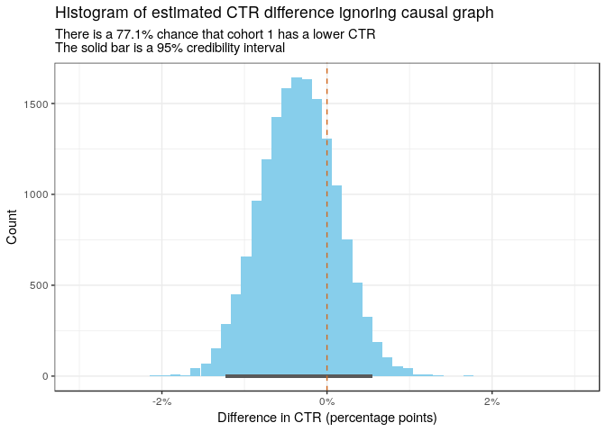
The problems outlined above are a direct result of ignoring the causal assumptions in our experimental setup.
Causal analysis
We can describe the problems above by drawing the causal diagrams for our assumptions. The correct causal diagram will then tell us how to get better estimates.
Causal diagrams
The causal model used in the previous section consists of only two nodes: cohort and click. This correctly assumes that cohort causes click but incorrectly assumes there are no confounders.

Although we intervene on cohort (there are no arrows into cohort), users can chose whether they take part in the experiments so we should model this self selection. The case we are interested in posits engagement as a confounder for viewing and clicking. We highlight view because our data are implicitly conditioned on users viewing the variant they were assigned.

Since we only have data for users who viewed the variants assigned to them, we know that these users are likely more engaged, and thus more likely to click. This explains why the naive analysis returns a CTR that is too high. Given that there is an interaction between engagement and cohort in our data, this also explains why the effect of the cohort is masked. In order to get to the parameters of interest, we need to make an adjustment.
The backdoor adjustment
Pearl+Co have shown that the backdoor adjustment can be applied in the above case - even in the presence of selection bias - given that we have external data about our population to estimate the the probability of engagement. The causal effect of \(X =\) cohort on \(Y=\) click is then
\[ \begin{align} \mathbb P (Y = 1 \mid \do(X = x)) &= \sum_{e=-1}^2 \mathbb P (Y = 1 \mid X = x, E = e, V = 1) \mathbb P(E = e) \\ &= \mathbb P (Y = 1 \mid X = x, E = -1, V = 1) \times 0.614 \\ &\mathbin{\hphantom{=}} + \mathbb P (Y = 1 \mid X = x, E = 0, V = 1) \times 0.325 \\ &\mathbin{\hphantom{=}} + \mathbb P (Y = 1 \mid X = x, E = 1, V = 1) \times 0.058 \\ &\mathbin{\hphantom{=}} + \mathbb P (Y = 1 \mid X = x, E = 2, V = 1) \times 0.003 \end{align} \]
where we have used the population frequency of the engagement segments for \(\mathbb P(E = e)\) (see below). Note that the probabilities we need to estimate can all be estimated from the observed data because they are all conditional on participation (\(V=1\)).
Causally modelling the data
Let’s get data aggregated on the level of cohort and segment.
xp <- xp_complete %>%
  filter(viewed) %>%
  group_by(cohort, segment) %>%
  summarise(
    views = n(),
    clicks = sum(clicked)
  )
We again fit a binomial model but this time include an estimate for the effect of segment and for the interaction of segment with the cohort. These extra features are indicated with the (1 + cohort | segment) notation. We did it this way instead of cohort * segment in order to allow partial pooling of estimates, which often improves the quality of estimates in segments with lower sample sizes (e.g. for the very highly engaged users).
model <- rstanarm::stan_glmer(
  # binomial test
  cbind(clicks, views - clicks) ~ 1 + cohort + (1 + cohort | segment),
  family = binomial(),
  data = xp,
  # same priors as before
  prior_intercept = prior_intercept,
  prior = prior,
  # MCMC sample sizes
  chains = 4,
  warmup = 1000,
  iter = 5000
)
In order to use the backdoor adjustment, we’ll need the relative frequencies of the segments in our general population.
population <- users %>%
  group_by(segment) %>%
  count() %>%
  ungroup() %>%
transmute(segment, weight = n / sum(n))| segment | weight |
|---|---|
| low | 0.613746 |
| medium | 0.324962 |
| high | 0.057928 |
| very_high | 0.003364 |
Now we can draw our Bayesian posterior estimates, then calculate the CTR for each cohort by taking the weighted average of CTR across the segments. Notice that the unobserved population averages now fall well within the credible intervals.
xp_draws_adjusted <- xp %>%
  select(cohort, segment) %>%
  tidybayes::add_fitted_draws(model) %>%
  as_tibble() %>%
  inner_join(population, by = 'segment') %>%
  mutate(adjusted = .value * weight) %>%
  group_by(cohort, .draw) %>%
summarise(ctr = sum(adjusted)) 
There is now no need to conduct any test on the difference because the two variants are so clearly different.