BDA3 Chapter 5 Exercise 4
Here’s my solution to exercise 4, chapter 5, of Gelman’s Bayesian Data Analysis (BDA), 3rd edition. There are solutions to some of the exercises on the book’s webpage.
Suppose we have \(2J\) parameters, of which \(J\) are \(\dnorm(1, 1)\) and the remaining \(J\) are \(\dnorm(-1, 1)\). These parameters are exchangeable since we have no way of knowing which are in the former group in which in the latter. Their exchangeable joint probability distribution would be the product of the \(2J\) independent normals averaged over all possible permutations.
Suppose we could write the joint distribution as a mixture of iid components
\[ p(\theta) = \int \prod_{j = 1}^J p(\theta_j \mid \phi) p(\phi) d\phi . \]
I won’t prove mathematically that his assumption leads to a contradiction, but rather simulate values to illustrate the point.
First, the solution to exercise 5 shows that the covariance of \(\theta_i, \theta_j\), \(i \ne j\), would have to be non-negative. So let’s simulate some values and take a look at the covariance.
rbern <- function(n, p) 2 * rbinom(n, 1, p) - 1

simulate <- function(J, iter = 10000) {
  tibble(
      mu1 = rbern(iter, 0.5),
      flip = rbern(iter, (J - 1) / (2*J - 1)),
      mu2 = mu1 * flip,
      theta1 = rnorm(iter, mu1, 1),
      theta2 = rnorm(iter, mu2, 1)
    )
}
In our simulate function, the flip variable indicates whether \(\theta_2\) has a mean that is the negative of the mean of \(\theta_1\). Notice that the probability of a flip depends on \(J\). In particular, when \(J = 1\) this probability is 1. For larger values of \(J\), the probability of a flip is strictly greater than 0.5. As \(J \to \infty\), this probability converges to 0.5, as if \(\theta_1\) and \(\theta_2\) were independent.

For this case where \(J = 1\), the correlation is clearly negative. We can also see two clusters forming around \((1, -1)\) and \((-1, 1)\). This seems reasonable since the mean of one is necessarily the negative of the mean of the other.
To see what happens when \(J \to \infty\), let’s calculate the covariance for a range of values of \(J\).
covariance <- function(sims)
  sims %>%
    summarise(cov(theta1, theta2)) %>%
    pull()

covariances <- tibble(J = 1:500) %>%
  mutate(
    sim = map(J, simulate),
    cov_theta1_theta2 = map_dbl(sim, covariance)
  )
We can see below that the covariance is quite negative for small values of \(J\), and it seems to converge very quickly to 0. I suspect the positive values that appear are due to sampling variance.
covariances %>%
  ggplot() +
  aes(J, cov_theta1_theta2) +
  geom_point(alpha = 0.4) +
  labs(y = 'Covariance')
Finally, let’s plot the samples for a large value of \(J\) to verify that there is (almost) no covariance.
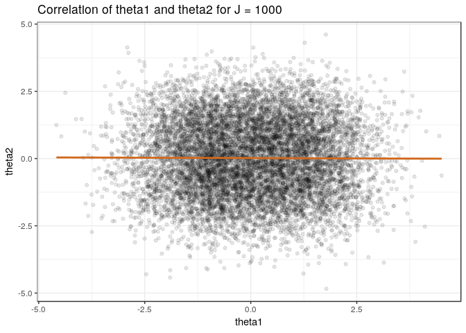
The covariance is negative for finite \(J\) since a large value of \(\theta_1\) implies it is most likely from \(\dnorm(1, 1)\), which implies that \(\theta_2\) is most likely from \(\dnorm(-1, 1)\) and would have a smaller value (and vice versa). This contradicts the assumption that we can write the joint distribution as a mixture of iids.
This doesn’t lead to a contradiction to de Finetti’s theorem by letting \(J \to \infty\) because the covariances converge to 0.