BDA3 Chapter 2 Exercise 12
Here’s my solution to exercise 12, chapter 2, of Gelman’s Bayesian Data Analysis (BDA), 3rd edition. There are solutions to some of the exercises on the book’s webpage.
Suppose \(\theta\) has a Poisson likelihood so that \(\log p(y \mid \theta) \propto y \log(\theta) - \theta\). We will find Jeffrey’s prior for \(\theta\) and the gamma distribution that most closely approximates it.
The derivative of the log likelihood is \(\frac{y}{\theta} - 1\) and the second derivative is \(-\frac{y}{\theta^2}\). It follows that the Fisher information for \(\theta\) is
\[ J(\theta) = \mathbb E \left( \frac{y}{\theta^2} \right) = \frac{1}{\theta} , \]
so Jeffrey’s prior is \(p(\theta) \propto \frac{1}{\sqrt{\theta}}\). This is an improper prior because
\[ \int_0^\infty \theta^{-\frac{1}{2}} d\theta = \left[ 2\theta^{\frac{1}{2}} \right]_0^\infty = \infty . \]
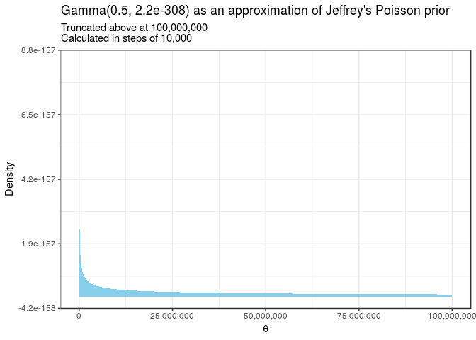
Since Jeffrey’s prior is improper, we can try approximate it with a gamma prior. Let \(\alpha, \beta \in (0, \infty)\) be the shape and rate parameters of a gamma distribution. Then
\[ \dgamma(\theta \mid \alpha, \beta) \propto x^{\alpha - 1}e^{-\beta x} . \]
Choosing \(\alpha = \frac{1}{2}\) and \(\beta = 0\) yields Jeffrey’s prior. However, \(\beta\) must be positive for the gamma distribution to be proper, so we can choose \(\beta = \epsilon\) sufficiently small. We’ll use the smallest positive float representable in R.
epsilon <- .Machine$double.xmin

upper_limit <- 100000000
step <- upper_limit / 10000

prior <- tibble(theta = seq(0, upper_limit, step)) %>%
  mutate(density = dgamma(theta, 0.5, epsilon))