BDA3 Chapter 2 Exercise 9
Here’s my solution to exercise 9, chapter 2, of Gelman’s Bayesian Data Analysis (BDA), 3rd edition. There are solutions to some of the exercises on the book’s webpage.
\(\DeclareMathOperator{\dbinomial}{binomial} \DeclareMathOperator{\dbern}{Bernoulli} \DeclareMathOperator{\dnorm}{normal} \DeclareMathOperator{\dgamma}{gamma} \DeclareMathOperator{\invlogit}{invlogit} \DeclareMathOperator{\logit}{logit} \DeclareMathOperator{\dbeta}{beta}\)
The data show 650 people in support of the death penalty and 350 against. We explore the effect of different priors on the posterior.
First let’s find the prior with a mean of 0.6 and standard deviation 0.3. The mean of the \(\dbeta(\alpha, \beta)\) distribution is
\[ \frac{3}{5} = \frac{\alpha}{\alpha + \beta} \]
which implies that \(\alpha = 1.5 \beta\). The variance is
\[ \begin{align} \frac{9}{100} &= \frac{\alpha \beta}{(\alpha + \beta)^2 (\alpha + \beta + 1)} \\ &= \frac{3}{2} \frac{\beta^2}{\frac{25}{4}\beta^2 \frac{5\beta + 2}{2}} \\ &= \frac{3}{2}\frac{4}{25}\frac{2}{5\beta + 2} \\ &= \frac{12}{25(5\beta + 2)} \\ &\Leftrightarrow \\ 5\beta + 2 &= \frac{12}{25}\frac{100}{9} \\ &= \frac{16}{9}, \end{align} \]
which implies that \(\beta = \frac{2}{3}\). Thus \(\alpha = 1\). Let’s check we’ve done the maths correctly.
α <- 1
β <- 2 / 3

list(
  'mean_diff' = 3 / 5 - α / (α + β),
  'variance_diff' = 9 / 100 - α * β / ((α + β)^2 * (α + β + 1))
)
## $mean_diff
## [1] -1.110223e-16
##
## $variance_diff
## [1] -1.387779e-17The value 1e-16 is computer-speak for 0.
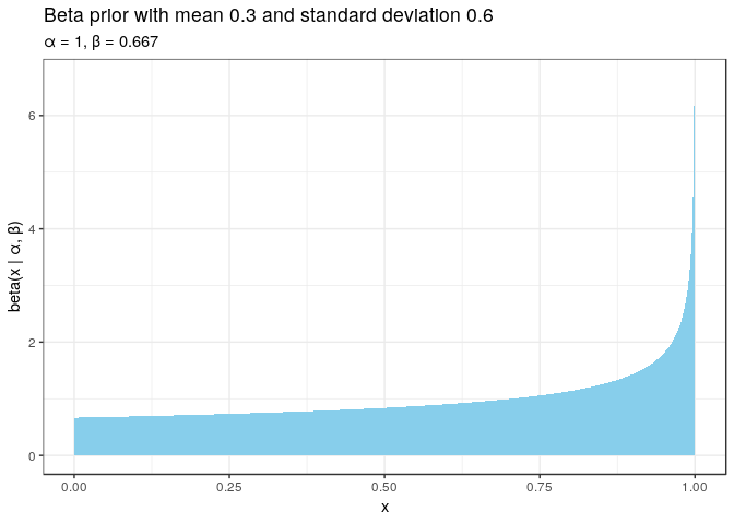
Since \(\beta < 1 <= \alpha\), we see one maximum at 1.
tibble(x = seq(0, 1, 0.001), y = dbeta(x, α, β)) %>%
  ggplot() +
  aes(x, y) +
  geom_area(fill = 'skyblue') +
  labs(
    x = 'x',
    y = 'beta(x | α, β)',
    title = 'Beta prior with mean 0.3 and standard deviation 0.6',
    subtitle = str_glue('α = {α}, β = {signif(β, 3)}')
  )
The beta distribution is self-conjugate so the posterior is \(\dbeta(0.6 + 650, 0.4 + 350)\).
Let’s plot the posterior with priors of different strength. We can increase the strength of the prior whilst keeping the mean constant by multiplying \(\alpha\) and \(\beta\) by the same constant c. We will use \(c \in \{ 1, 10, 100, 1000\}\). In the plot below, we have restricted the x-axis to focus on the differences in the shape of the posteriors.
support <- 650
against <- 350

expand.grid(magnitude = 0:3, x = seq(0, 1, 0.001)) %>%
  as_tibble() %>%
  mutate(
    c = 10^magnitude,
    a_prior = α * c,
    b_prior = β * c,
    y = dbeta(x, support + a_prior, against + b_prior),
    prior_magnitude = factor(as.character(10^magnitude))
  ) %>%
  ggplot() +
  aes(x, y, colour = prior_magnitude) +
  geom_line() +
  scale_x_continuous(limits = c(0.55, 0.75)) +
  labs(
    x = 'x',
    y = 'beta(x | support + a, against + b)',
    title = 'Beta posterior with different priors',
    subtitle = str_glue(paste(
      'a = {α} * 10^magnitude, b = {β} * 10^magnitude',
      'support = 650, against = 350',
      sep = '\n'
    )),
    colour = 'Magnitude of the prior'
  )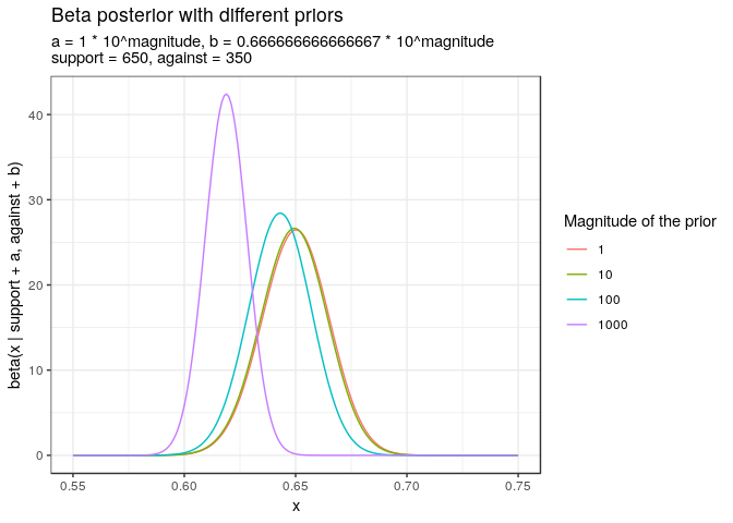
Magnitudes 1 and 10 give very similar results close to the maximum likelihood estimate of 65%. The higher magnitudes pull the mean towards the prior mean of 60%.