BDA3 Chapter 2 Exercise 4

Posted on 23 August, 2018 by Brian
Tags: binomial, bayes, solutions, bda chapter 2, bda, normal approximation, multi-modal
Category: bda3

Here’s my solution to exercise 4, chapter 2, of Gelman’s Bayesian Data Analysis (BDA), 3rd edition. There are solutions to some of the exercises on the book’s webpage.

Consider 1000 rolls of an unfair die, where the probability of a 6 is either 1/4, 1/6, or 1/12. Let’s draw the distribution and the normal approximation.

N <- 1000
p6 <- c(1 / 4, 1 / 6, 1 / 12)

ex4 <- expand.grid(
    y = seq(0, N),
    theta = p6
  ) %>% 
  mutate(
    mu = N * theta,
    sigma = sqrt(N * theta * (10 - theta)),
    binomial = dbinom(y, N, theta),
    normal_approx = dnorm(y, mu, sigma),
    theta = scales::percent(signif(theta))
  ) %>% 
  select(-mu, -sigma) %>% 
  gather(distribution, probability, binomial, normal_approx) %>% 
  spread(theta, probability) %>% 
  mutate(prior_probability = 0.25 * `8.3%` + 0.5 * `16.7%` + 0.25 * `25.0%`)

y	distribution	16.7%	8.3%	prior_probability
0	binomial	0.0e+00	0.0000000	0.00e+00
0	normal_approx	2.1e-06	0.0002078	5.30e-05
1	binomial	0.0e+00	0.0000000	0.00e+00
1	normal_approx	2.3e-06	0.0002297	5.86e-05
2	binomial	0.0e+00	0.0000000	0.00e+00
2	normal_approx	2.5e-06	0.0002536	6.47e-05

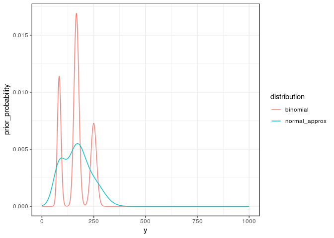
The normal approximation underestimates the maxima and overestimates the values between the maxima. From the percentiles in the table below, we see that the normal approximation is best near the median but becomes gradually worse towards towards both extremes.

percentiles <- c(0.05, 0.25, 0.5, 0.75, 0.95)

ex4 %>% 
  group_by(distribution) %>% 
  arrange(y) %>% 
  mutate(
    cdf = cumsum(prior_probability),
    percentile = case_when(
      cdf <= 0.05 ~ '05%',
      cdf <= 0.25 ~ '25%',
      cdf <= 0.50 ~ '50%',
      cdf <= 0.75 ~ '75%',
      cdf <= 0.95 ~ '95%'
    )
  ) %>% 
  filter(cdf <= 0.95) %>% 
  group_by(distribution, percentile) %>% 
  slice(which.max(cdf)) %>% 
  select(distribution, percentile, y) %>% 
  spread(distribution, y) %>% 
  arrange(percentile) %>% 
  kable() %>% kable_styling()

percentile	binomial	normal_approx
05%	75	58
25%	119	110
50%	166	164
75%	206	214
95%	260	291