BDA3 Chapter 2 Exercise 3
Here’s my solution to exercise 3, chapter 2, of Gelman’s Bayesian Data Analysis (BDA), 3rd edition. There are solutions to some of the exercises on the book’s webpage.
For 1000 rolls of a fair die, The mean number of sixs is 1000/6 = 166.667, the variance is 138.889, and the standard deviation is 11.7851. Let’s compare the binomial distribution to the normal approximation.
N <- 1000
p <- 1 / 6
mu <- N * p
sigma <- sqrt(N * p * (1 - p))

ex3 <- tibble(
    y = seq(0, N),
    binomial = dbinom(y, N, p),
    normal_approx = dnorm(y, mu, sigma)
  ) %>%
gather(metric, probability, -y) | y | metric | probability |
|---|---|---|
| 0 | binomial | 0 |
| 1 | binomial | 0 |
| 2 | binomial | 0 |
| 3 | binomial | 0 |
| 4 | binomial | 0 |
| 5 | binomial | 0 |
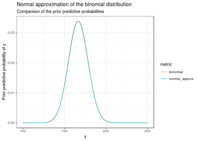
The two curves are visually indistinguishable. The percentiles are listed in the table below.
percentiles <- c(0.05, 0.25, 0.5, 0.75, 0.95)

tibble(
    percentile = scales::percent(percentiles),
    binom = qbinom(percentiles, N, p),
    norm = qnorm(percentiles, mu, sigma)
) %>% kable() %>% kable_styling()| percentile | binom | norm |
|---|---|---|
| 5% | 147 | 147.2819 |
| 25% | 159 | 158.7177 |
| 50% | 167 | 166.6667 |
| 75% | 175 | 174.6156 |
| 95% | 186 | 186.0515 |