BDA3 Chapter 2 Exercise 1

Here’s my solution to exercise 1, chapter 2, of Gelman’s Bayesian Data Analysis (BDA), 3rd edition. There are solutions to some of the exercises on the book’s webpage.

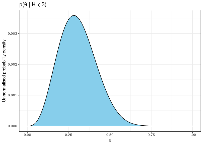
Let H be the number of heads in 10 tosses of the coin. With a beta(4,4) prior on the probability θ of a head, the posterior after finding out H≤2 is

p(θ∣H≤2)∝p(H≤2∣θ)⋅p(θ)=beta(θ∣4,4)2∑h=0binomial(h∣θ,10)=θ3(1−θ)32∑h=0(10h)θh(1−θ)10−h.

We can plot this unnormalised posterior density from the following dataset.

ex1 <- tibble(
         theta = seq(0, 1, 0.01), 
         prior = theta^3 * (1 - theta)^3,
         posterior = prior * (
           choose(10, 0) * theta^0 * (1 - theta)^10 +
           choose(10, 1) * theta^1 * (1 - theta)^9 +
           choose(10, 2) * theta^2 * (1 - theta)^8 
         )
       )

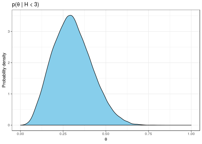
With the help of Stan, we can obtain the normalised posterior density. We include the information that there are at most 2 heads observed by using the (log) cumulative density function.

m1 <- rstan::stan_model('src/ex_02_01.stan')

S4 class stanmodel 'ex_02_01' coded as follows:
transformed data {
  int tosses = 10;
  int max_heads = 2;
}

parameters {
  real<lower = 0, upper = 1> theta;
}

model {
  theta ~ beta(4, 4); // prior 
  target += binomial_lcdf(max_heads | tosses, theta); // likelihood
} 

The following posterior has the same shape as our exact unnormalised density above. The difference is that we now have a normalised probability distribution without having to work out the maths ourselves.

f1 <- sampling(m1, iter = 40000, warmup = 500, chains = 1)